Graph Data Structures

At the core of TorchDrug, we provides several data structures to enable common operations in graph representation learning.

Create a Graph

To begin with, let’s create a graph.

import torch
from torchdrug import data

edge_list = [[0, 1], [1, 2], [2, 3], [3, 4], [4, 5], [5, 0]]
graph = data.Graph(edge_list, num_node=6)
graph.visualize()

This will plot a ring graph like the following.

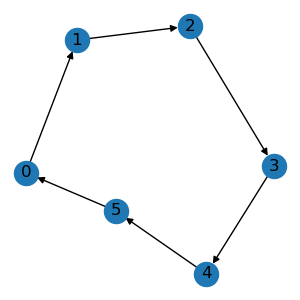
Internally, the graph is stored as a sparse edge list to save memory footprint. For an intuitive comparison, a scale-free graph may have 1 million nodes and 10 million edges. The dense version takes about 4TB, while the sparse version only requires 120MB.

Here are some commonly used properties of the graph.

print(graph.num_node)
print(graph.num_edge)
print(graph.edge_list)
print(graph.edge_weight)

In some scenarios, the graph may also have type information on its edges. For example, molecules have bond types like single bound, while knowledge graphs have relations like consists of. To construct such a relational graph, we can pass the edge type as a third variable in the edge list.

triplet_list = [[0, 1, 0], [1, 2, 1], [2, 3, 0], [3, 4, 1], [4, 5, 0], [5, 0, 1]]
graph = data.Graph(triplet_list, num_node=6, num_relation=2)
graph.visualize()

Alternatively, we can also use adjacency matrices to create the above graphs.

The normal graph uses a 2D adjacency matrix \(A\), where non-zero \(A_{i,j}\) corresponds to an edge from node \(i\) to node \(j\). The relational graph uses a 3D adjacency matrix \(A\), where non-zero \(A_{i,j,k}\) denotes an edge from node \(i\) to node \(j\) with edge type \(k\).

adjacency = torch.zeros(6, 6)
adjacency[edge_list] = 1
graph = data.Graph.from_dense(adjacency)

adjacency = torch.zeros(6, 6, 2)
adjacency[triplet_list] = 1
graph = data.Graph.from_dense(adjacency)

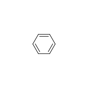
For molecule graphs, TorchDrug supports creating instances from SMILES strings. For example, the following code creates a benzene molecule.

mol = data.Molecule.from_smiles("C1=CC=CC=C1")
mol.visualize()

Once the graph is created, we can transfer it between CPU and GPUs, just like torch.Tensor.

graph = graph.cuda()
print(graph.device)

graph = graph.cpu()
print(graph.device)

Graph Attributes

A common practice in graph representation learning is to add some graph features as the input of neural networks. Typically, there are three types of features, node-level, edge-level and graph-level features. In TorchDrug, these features are stored as node/edge/graph attributes in the data structure, and are automatically processed during any graph operation.

Here we specify some features during the construction of the molecule graph.

mol = data.Molecule.from_smiles("C1=CC=CC=C1", atom_feature="default",
                                bond_feature="default", mol_feature="ecfp")
print(mol.node_feature.shape)
print(mol.edge_feature.shape)
print(mol.graph_feature.shape)

There are a bunch of popular feature functions provided in torchdrug.data.feature. We may also want to define our own attributes. This only requires to wrap the assignment lines with a context manager. The following example defines edge importance as the reciprocal of node degrees.

node_in, node_out = mol.edge_list.t()[:2]
with mol.edge():
    mol.edge_importance = 1 / graph.degree_in[node_in] + 1 / graph.degree_out[node_out]

We can use mol.node() and mol.graph() for node- and graph-level attributes respectively. Attributes may also be a reference to node/edge/graph indexes. See Deal with References for more details.

Note in order to support batching and masking, attributes should always have the same length as their corresponding components. This means the size of the first dimension of the tensor should be either num_node, num_edge or 1.

Batch Graph

Modern deep learning frameworks employs batched operations to accelerate computation. In TorchDrug, we can easily batch same kind of graphs with arbitary sizes. Here is an example of creating a batch of 4 graphs.

graphs = [graph, graph, graph, graph]
batch = data.Graph.pack(graphs)
batch.visualize(num_row=1)

This returns a PackedGraph instance with all attributes automatically batched. The essential trick behind this operation is based on a property of graphs. A batch of \(n\) graphs is equivalent to a large graph with \(n\) connected components. The equivalent adjacency matrix for a batch is

\[\begin{split}A = \begin{bmatrix} A_1 & \cdots & 0 \\ \vdots & \ddots & \vdots \\ 0 & \cdots & A_n \end{bmatrix}\end{split}\]

where \(A_i\) is the adjacency of \(i\)-th graph.

To get a single graph from the batch, use the conventional index or PackedGraph.unpack.

graph = batch[1]
graphs = batch.unpack()

One advantage of such batching mechanism is that it does not distinguish a single graph and a batch. In other words, we only need to implement single graph operations, and they can be directly applied as batched operations. This reduces the pain of writing batched operations.

Subgraph and Masking

The graph data structure also provides a bunch of slicing operations to create subgraphs or masked graphs in a sparse manner. Some typical operations include

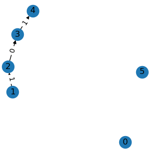
g1 = graph.subgraph([1, 2, 3, 4])
g1.visualize()

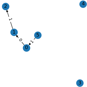
g2 = graph.node_mask([1, 2, 3, 4])
g2.visualize()

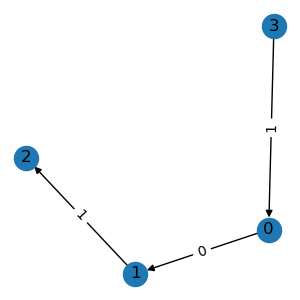
g3 = graph.edge_mask([0, 1, 5])
g3.visualize()

g4 = g3.compact()
g4.visualize()

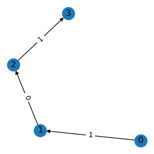
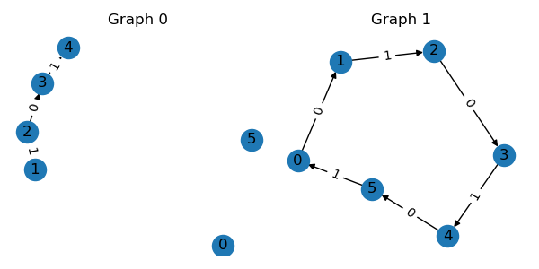
All the above operations accept either integer node indexes or binary node masks. subgraph() extracts a subgraph based on the given nodes. The node ids are re-mapped to produce a compact index. node_mask() keeps edges among the given nodes. edge_mask() keeps edges of the given edge indexes. compact() removes all isolated nodes.

The same operations can also be applied to batches. In this case, we need to convert the index of a single graph into the index in a batch.

graph_ids = torch.tensor([0, 0, 0, 0, 1, 1, 1, 1, 1, 1])
node_ids = torch.tensor([1, 2, 3, 4, 0, 1, 2, 3, 4, 5])
node_ids += batch.num_cum_nodes[graph_ids] - batch.num_nodes[graph_ids]
batch = batch.node_mask(node_ids)
batch.visualize(num_row=1)

We can also pick a subset of graphs in a batch.

batch = batch[[0, 1]]
batch.visualize()